Expecting Goals: Across Time & Space
At the confluence of football and data
In Spring 2024, the three of us — Karnav, Pranav and Suyog — all undergraduate students of computer science at Ashoka University, undertook an independent study module to study the applications of predictive machine learning in football. We used freely available data from StatsBomb to replicate their industry-leading goal-prediction model and looked for patterns in the data to support or refute our sporting intuition. In Part 1 of this blog series, we outline all that we did and all that we found — some of which surprised us quite a bit!
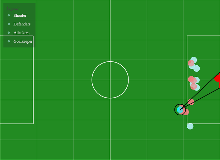
Note: All of our code is available for use and replication at https://github.com/kkkarnav/betterxG. For those with an interest in data science and football, we highly encourage you to explore our work and see if you find something interesting!
What are expected Goals?
Data analytics in football is a field almost as old as the sport itself. The first football analysts are considered to be Charles Reep and Bernard Benjamin all the way back in the 1960s, who watched hundreds of matches to manually analyze which types of shots and positions most often resulted in goals. Their collaborator, Charles Hughes, created the first football metric: Position of Maximum Opportunity. This simplistic metric measured the likelihood of a goal purely from the position on the pitch that the shot was taken from.
As the Premier League globalized football and scouts and analysts started playing a greater role in team strategy, football analytics grew much more sophisticated, though still informal. The first use of the phrase “expected goals”, though not in modern context, was in Vic Barnett and Sarah Hilditch’s 1993 paper “The Effect of an Artificial Pitch Surface on Home Team Performance in Football (Soccer)”, which performed a regression analysis of the impact of artificial pitches on goals. Meanwhile, scouts had begun identifying lists of factors that influence the likelihood of a goal, including angle, pressure, and form.
Expected Goals as a formal metric for football performance came into existence in 2012, during a time of increased interest in statistical measurement of football due to the proliferation of blog posts as a popular forum for sports analysts. Sam Green, an analyst at OptaPro, first described the xG metric in April 2012, which revolutionized the football analytics industry. Since then, xG has become more and more complex, both by taking into account more features, as well as by fine tuning the representation of important features to best capture the reality on the pitch.
What data will we use to model xG?
To replicate StatsBomb’s (extensively documented) xG model, we’ll use a variety of ML models and techniques combined with extensive feature engineering and finetuning on as much granular data as we can find. The best and most detailed source of football event data is from the StatsBomb data collection platform, which uses computer vision and detailed match footage to generate extensive event data. StatsBomb is a market-leading sports data & analytics firm, particularly in football. Its Expected Goals (xG) and On-Ball Value (OBV) models are cutting-edge in the field and typically outperform competitors by a significant margin, largely because of the greater volume and variety of data available via StatsBomb’s data pipeline.
While StatsBomb data is proprietary (and exorbitantly expensive), it has made a subset of its data available freely through its Open Data project. StatsBomb Open Data consists of one full season (2015/16) of data across the top 5 European leagues, as well as a variety of smaller sets of data from the Mens’ and Womens’ World Cups and Euros, Lionel Messi’s career, and African Cup of Nations, among others. In total, event data from more than 3500 matches across 21 competitions has been made available. This provides a significant amount of data on which prediction algorithms can be trained and tested.
We can access and load the Open Data through the StatsBomb API via the statsbombpy package in Python. This allows us to load a flat dataset containing 11.6 million observations — events of all types from more than 3500 matches across 40 seasons and 21 competitions. Of course, our analysis will most be restricted to shots (and goals), for which we’ll construct a dataframe of 83,929 shots from the 3312 matches included in our analysis.

How will we model xG?
What we’ll want to do now is regress on this data to accurately predict the likelihood of a shot becoming a goal. Note that while this is nominally a classification problem, what we really want is xG, which is equivalent to the likelihood of the data point being assigned to the minority class. As a result, we’ll implement both linear and logistic regression (as a sanity check). We’ll then implement three decision-tree-based models, which are the state-of-the-art in xG. The first is a regular decision tree, while the other two are two ensemble models — random forest and extreme gradient boosted classification.
The first thing we’ll do is simply throw the data into the model and see how it compares to StatsBomb’s official xG figures, without any preparation or engineering. Based on our literature review, we expected the xGBoost tree to do the best, and it does turn out to be so. At the optimal threshold, xGBoost achieves an F1 score of 37 and an accuracy of 88%, significantly better than our other options. StatsBomb’s own predicted xG comes in at 40 F1, quite a bit better than us.
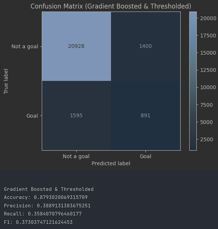

StatsBomb is better than us at almost every threshold value, which we can conclude based on our F1 scores across thresholds and the ROC curves. There’s a lot of scope for us to improve.


Next Steps
To augment our analysis, we’ll spend a lot of time improving our models on two fronts — the football side, and the data and machine learning side. On the football side, we’ll attempt to engineer new features based on StatsBomb’s data that better explain footballing situations. We’ll go into more detail on the process of this in Part 2. On the data and machine learning side, we’ll dive deep into the data and use some of the common techniques available to develop our model’s capabilities. We’ll cover the nuts and bolts of this in Part 3.
At the end of it all, we’ll have our final model, with new features and new parameters. Let’s see how it does!

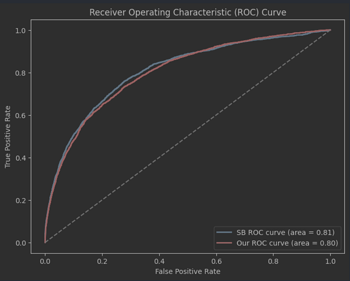
As expected, xGBoost is still our best model, and we can see that it is now a lot closer to the “official” StatsBomb values, achieving an F1 score of 40 and an accuracy of 87%. On all of our metrics, we are now within 1% of StatsBomb. The remaining 1% can probably accounted for by the fact that StatsBomb has access to a lot (hundreds of times as much) more data than us.
Looking at the F1 scores and the ROC curve tells the same story — we’re now acceptably close to the industry-standard models to call it a success.

Now for the interesting part. What insights can we draw from our newly interpretable prediction model? Let’s put some common football hypotheses to the test.
The Clock Is Ticking
The first common football intuition that we want to examine is — does time matter in a game? Football fans will know that every close game has spells of dominance for both sides — phases of play where a team can’t get out of their own half, and phases where they have a shot practically every minute. The last minutes of the game, particularly in close games, are also seen very differently from the rest of the match. This is when teams tend to take many high-variance shots, hoping to get lucky. There are non-statistical rationalizations for this — as the match goes on, defenders get more tired, shooters get frustrated, the pressure increases, and so on. Similarly, if your team is dominating the state of play, you’ll play more confidently, be riskier, back yourself more than usual.
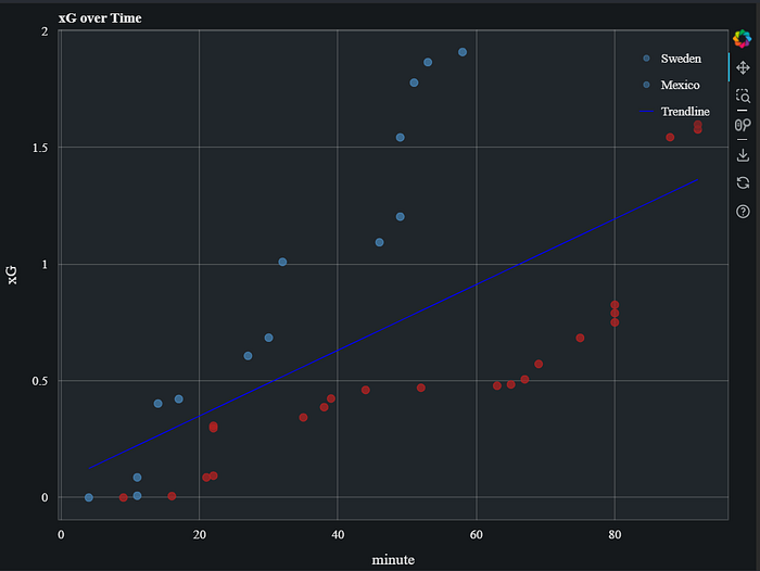
Does this perception hold up to statistical rigour? Specifically, does the time of the match, or the dominance in the last few minutes of play, make a difference to the likelihood of scoring?
At a cursory glance, it would appear not — the mutual information between our target variable (whether it’s a goal or not) and our various measures of time patterns (whether it’s extra time, how many shots there have been in the past 15 minutes, how many shots there have been so far) is almost 0 — indicating that they explain none of the variation in whether a shot becomes a goal or not. The only exception is the number of shots by the same team in the past minute — that probably covers scenarios where the ball falls loose in the box or comes off the goalie and is poked in.
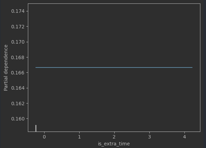

However, our hypothesis is not that these metrics are significant determinants of goals in general, but rather that they account for variations only in certain scenarios. A good check would therefore be to see if our decision tree picks up on any of these metrics.
No respite for the time pattern hypothesis — none of the time-based features feature in our tree, even when we turn the maximum depth up to 12. We can conclude fairly confidently that the time of the match when you take the shot doesn’t seem to change likelihood too much.
Fair Weather Scorers
A linked but different hypothesis says that what matters more, from a psychological perspective, is whether the shooter’s team is leading or not. A team under the pressure of losing a critical game will probably behave quite differently from a team that’s leading by 5 goals. Immediately, the data doesn’t seem to support this line of thinking quite a bit more — mutual information indicates that the number of goals the team is leading by, and whether they are leading or trailing, account for 0.1 and 0.4% of the variation of our target variable.

When we take a look at the tree though — it tells an entirely different story. The tree picks up on the indicator of whether the team is leading or trailing twice, though it doesn’t seem to be integral. This makes intuitive sense — the psychological weight of leading or trailing should be the difference maker in tight situations. We can therefore chalk this down to a (somewhat) confirmed hypothesis.
Lefties Against Lefties
Something else that we were very interested in is the (now quite conventional) trend of playing right-footed left wingers and vice-versa. While in bygone eras the wingers were supposed to stick to the touchline, and therefore favour their outer foot, the cut-inside-and-shoot mentality of today requires a different skillset. Therefore, what we’d like to examine is whether there’s a statistically significant effect of a player shooting from the favoured side for their foot. While we have no data for player footedness, we can formulate this simply as — is a shot from the left foot from the right side of the pitch better or worse than a left-footed shot from the left side?

Mutual information is once again somewhat inconclusive — the footedness accounts for 0.7% of the variation in whether the shots converts or not, but the tree once again settles things. The feature ends up never being used, settling things in favour of the modern practice. It would appear that the side of the pitch and the footedness of a shot make little difference — a left footed shot is no more likely to convert whether it’s taken from the left side of the pitch or the right. While this obviously doesn’t control for the footedness of the player nor the differing frequencies with which each type of shot might be taken, it does lend some credence to players being able to handle a wider variety of shooting situations.
When In Rome
The last hypothesis we had, which is well-established in the literature, is that different leagues have different styles of play. That is to say, the types of shots that are taken in, for example, the German Bundesliga are very different from the types of shots that are taken in the Spanish Liga. We can reduce this to the problem of testing whether the two leagues have the same distribution; if so, we’d expect a model trained on one league to perform equally well on both of them.
We ran four experiments to establish this: training and testing within leagues (baseline), and training on one league and testing on the other. We repeated each experiment 100 times and measured performance using F1 scores, and found that there was a small reduction in performance when testing outside the league we trained on. Since the difference was small, we ran tests to ensure that the differences were statistically significant. These tests confirmed that the differences were not due to chance.
We can then conclude two things — that the model struggled to generalize to new, unseen data, and that there are striking differences in the quality of teams and the playstyles between German and Spanish football. This was as expected — the German league tends to be heavily counterattacking, while the Spanish league is much more technical. However, to be able to see this difference statistically in the shots from each league points to how stark the difference is, and how our model can pick up subtle patterns in the data.
The End
That concludes most of our results and learnings. The entire exercise was an immense learning experience for all of us — in terms of both machine learning as well as the sport. We were quite surprised to reach as close to StatsBomb’s performance baseline as we did, a testament to the quality of their data and their commitment to openness. The models we trained, and the hypotheses we were resultantly able to test, are a great start to a long-standing passion project, and we’d love for people to contribute in their own areas of interest. We hope that our work serves as a good base for future efforts in football analytics.
